Spalart–Allmaras turbulence model
The Spalart–Allmaras model is a one equation model for the turbulent viscosity. It solves a transport equation for a viscosity-like variable  . This may be referred to as the Spalart–Allmaras variable.
Contents |
Original model
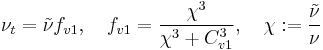
The turbulent eddy viscosity is given by
![\frac{\partial \tilde{\nu}}{\partial t} %2B u_j \frac{\partial \tilde{\nu}}{\partial x_j} = C_{b1} [1 - f_{t2}] \tilde{S} \tilde{\nu} %2B \frac{1}{\sigma} \{ \nabla \cdot [(\nu %2B \tilde{\nu}) \nabla \tilde{\nu}] %2B C_{b2} | \nabla \nu |^2 \} - \left[C_{w1} f_w - \frac{C_{b1}}{\kappa^2} f_{t2}\right] \left( \frac{\tilde{\nu}}{d} \right)^2 %2B f_{t1} \Delta U^2](/2012-wikipedia_en_all_nopic_01_2012/I/476216889d1ea0604979b921eae3428c.png)
![f_w = g \left[ \frac{ 1 %2B C_{w3}^6 }{ g^6 %2B C_{w3}^6 } \right]^{1/6}, \quad g = r %2B C_{w2}(r^6 - r), \quad r \equiv \frac{\tilde{\nu} }{ \tilde{S} \kappa^2 d^2 }](/2012-wikipedia_en_all_nopic_01_2012/I/09b19885ed6dffe3dec850e2516f1696.png)
![f_{t1} = C_{t1} g_t \exp\left( -C_{t2} \frac{\omega_t^2}{\Delta U^2} [ d^2 %2B g^2_t d^2_t] \right)](/2012-wikipedia_en_all_nopic_01_2012/I/993b41d0ba795e0b3877d041c4cff1cb.png)
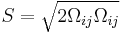
The rotation tensor is given by
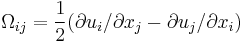
and d is the distance from the closest surface.
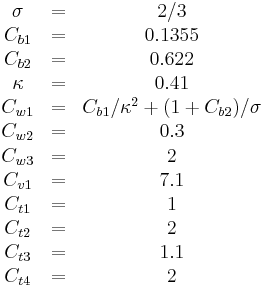
The constants are
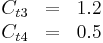
Modifications to original model
According to Spalart it is safer to use the following values for the last two constants:
Other models related to the S-A model:
DES (1999) [1]
DDES (2006)
Model for compressible flows
There are two approaches to adapting the model for compressible flows. In the first approach the turbulent dynamic viscosity is computed from

where  is the local density. The convective terms in the equation for are modified to
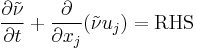
where the right hand side (RHS) is the same as in the original model.
Boundary conditions
Walls: 
Freestream:
Ideally , but some solvers can have problems with a zero value, in which case  can be used.
This is if the trip term is used to "start up" the model. A convenient option is to set  in the freestream. The model then provides "Fully Turbulent" behavior, i.e., it becomes turbulent in any region that contains shear.
Outlet: convective outlet.
References
- Spalart, P. R. and Allmaras, S. R., 1992, "A One-Equation Turbulence Model for Aerodynamic Flows" AIAA Paper 92-0439
External links
- This article was based on the Spalart-Allmaras model article in CFD-Wiki
- What Are the Spalart-Allmaras Turbulence Models? from kxcad.net
- The Spalart-Allmaras Turbulence Model at NASA's Langley Research Center Turbulence Modelling Resource site